A hundred ways to skin a cat – or some practical thoughts on benchmark replication
Juliusz Jabłecki and Jacek Próchniak
Executive summary
Trends in reserve management: 2020 survey results
Interview: Ma. Ramona Santiago
Scoring climate risks: which countries are the most resilient?
A hundred ways to skin a cat – or some practical thoughts on benchmark replication
Developing a sovereign ALM framework: a case study of Mauritius
Developing an integrated information system for reserve management: the experience of Peru
Appendix 1: Survey questionnaire
Appendix 2: Survey responses and comments
Appendix 3: Reserve statistics
The cornerstone of any reserve manager’s strategic asset allocation is the selection of a benchmark – ie, a portfolio that represents the institution’s mandate, long-term risk/return preferences and general investment guidelines (see, for instance, Box 4.1). Choosing a benchmark is critical as it typically determines the lion’s share of the variance of actual portfolio returns.
In the fixed income space, benchmarks tend to either be made up of one or several readily available broad bond indices compiled by investment banks and other external providers, or constructed in-house to more closely match an institution’s specific needs and requirements (investment universe, risk limits, etc). Whichever approach is ultimately chosen, once a benchmark is selected it needs to be implemented – ie, a replicating portfolio needs to be built and maintained over time. The latter task is entrusted to portfolio managers who are therefore responsible not only for ensuring that an institution’s broad investment vision is realised in practice, but are often also allowed to position vis-à-vis the benchmark in an attempt to modestly add value to the investment process.
The irony here is that while the determination of the strategic benchmark ends up being responsible for most of the risk inherent in the foreign exchange reserves portfolio (about 90%), it normally consumes only about 10% of the institution’s overall resources. Conversely, while building, maintaining and positioning the portfolios against the benchmark adds little total risk, it consumes the vast majority of the institution’s time and effort. This disparity is very well reflected in the academic and professional literature, which mostly focuses on strategic asset allocation and choosing an optimal benchmark, whereas the bread and butter of tactical portfolio management attracts considerably less attention. There are, it seems, few general guidelines to follow, and no readily available industry best practices to consult on how to optimally construct a portfolio replicating some optimally designed benchmark. And yet, benchmark replication can hardly be disregarded as too “technical” and “operational” to be a subject of rigorous treatment.
Box 4.1 Reserve management at Narodowy Bank Polski
Foreign exchange (FX) reserves held by Narodowy Bank Polski (NBP) are invested in a three-stage process that sets asset allocation at strategic, tactical and operational levels. The first stage determines the absolute level of exposure to major risks, which in terms of foreign exchange risk is given by the currency structure and for interest rate risk by the modified duration of individual portfolios. These parameters constitute the “strategic benchmark”, and are approved by the management board each year. The “tactical benchmark”, which is reviewed from time to time by an investment committee, allows for medium-term adjustments to the main exposures and is expressed with regard to relative deviations from the strategic benchmark. In turn, the tactical benchmark is a reference for portfolio managers that conduct the day-to-day operations of investing and trading.
While both benchmarks are formally set as a combination of parameters, practical reasons require them to be expressed in the form of portfolios consisting of actual instruments. These benchmark portfolios are constructed by the middle office, and are rebalanced at the beginning of each month to maintain a stable duration exposure. The list of instruments and their respective weights for a given month is prepared according to a set of rules, the purpose of which is to make the benchmark a good representation of securities available on the market while also avoiding instruments that may be of limited availability or liquidity. The main purpose of benchmark portfolios is to provide rates of return that can be used to assess the effectiveness of strategic and tactical allocations, as well as the excess return generated by the portfolio managers.
With this in mind, we offer the following thoughts, which although by no means exhaustive will hopefully shed some light on the key issues and tradeoffs related to replicating fixed income benchmarks, bringing the topic of tactical portfolio management from the background to the foreground. The first section examines these issues from the perspective of a central bank investing in government bond markets. The next section then assesses bond index replication, particularly bond-by-bond replication based on matching exactly individual benchmark positions and replication based on matching the benchmark’s risk exposures. The third section looks at potential problems of yield-maximising replicating portfolios, such as their leanness making them very concentrated, and the issue of portfolio turnover. The following section discusses the use of derivatives to mitigate uncompensated transaction costs which are borne by portfolio managers but are not reflected in the benchmark, and how a simple rule-based risk-exposure replication could allows the portfolio to track the benchmark with acceptable accuracy. A final section provides some concluding remarks.
Setting the stage: problems and trade-offs
As hinted above, a fixed income benchmark portfolio will typically be based on either one or several indices, and as such comprises a broad selection of debt instruments representative of a given market segment. For example, given an allocation to the USD market with a duration target of around two – which seems to be the most common choice among reserve managers11 Nick Carver and Robert Pringle (Eds), HSBC Reserve Management Trends 2019 (London: Central Banking Publications, 2019). – and a distaste for bonds with maturities longer than ten years, one could either opt for an available Treasury index (ICE BofA1–3 Year or 0–5 Year Treasury: both offer a modified duration of around two) or a use a combination of several indices. The latter approach allows for a more complex allocation of securities across the yield curve, which may benefit the risk/return profile by increasing the convexity and, in some cases, the yield of the portfolio. As discussed above, the chosen benchmark becomes the reference for managers tasked with building and maintaining an actual fixed income portfolio (see Box 4.2).
Box 4.2 Fixed income indices
The indexing industry offers a constantly expanding selection of benchmarks. In the fixed income space, these range from broad representations of entire markets to small and specialised indices containing securities that satisfy certain, often detailed, criteria. As such, the number of instruments in an index may vary from many thousands (eg, more than 16,000 in the MSCI US Broad Market Index) to dozens or only a few (eg, the Norway Government Index currently consists of eight securities). Since the risk characteristics of fixed income securities change over time and most of them eventually mature, the composition of indices needs to be regularly updated and rebalanced, which can make the process of tracking them significantly more challenging than in the case of, say, equity indices (see Table 4.1).
| Number of instruments | Effective duration | Market value | Minimum yield (%) | Average yield (%) | Maximum yield (%) | Average rebalancing effective duration change | |
| 31 December 2019 | 2010–19 | ||||||
| ICE BofA US Broad Market | 16,211 | 6.07 | $27.6 trillion | 1.0 | 2.8 | 15.5 | +0.08 |
| ICE BofA US Broad Credit | 9,207 | 7.43 | $8.8 trillion | 1.2 | 2.9 | 7.7 | +0.08 |
| ICE BofA US Treasury | 260 | 6.70 | $11.2 trillion | 1.6 | 1.8 | 2.4 | +0.09 |
| ICE BofA 0–5 Year US Treasury | 202 | 2.15 | $7.9 trillion | 1.6 | 1.6 | 1.8 | +0.09 |
| ICE BofA Euro Government | 366 | 8.27 | €6.7 trillion | –0.7 | 0.2 | 2.6 | +0.08 |
| Source: ICE; Bloomberg. | |||||||
The key concept, and arguably the very starting point of this more tactical part of the investment process, is replication: a practice that essentially aims to mimic the behaviour of the benchmark, and specifically its risk and return profile. While portfolio management styles are often labelled passive or active depending on the degree of deviation from the benchmark’s risk/return profile, it is important to recognise that both approaches are defined relative to the benchmark, and in fact cannot be effectively or consistently executed without a clear picture of benchmark portfolio characteristics. Broadly speaking, these characteristics can be captured either by matching the benchmark on a bond-by-bond basis – ie, holding exactly the same securities with exactly the same weights as the benchmark, what we might call “perfect replication” – or by focusing instead on the benchmark’s overall risk measures (duration, convexity, etc) and aiming to build a leaner proxy portfolio with perhaps fewer total positions, but the same or similar risk exposure.
Some benchmarks may be perfectly replicated with little difficulty (for a Norwegian government bond index, it requires purchasing sufficient amount of eight issues), while for others the task could be almost impossible (consider indices consisting of thousands of individual issues or with large changes in composition).22 In January 2020, the ICE BofA US Broad Market index consisted of 16,211 individual securities, 253 of which were added in the December/January rebalancing (183 securities were removed). For managers pursuing a passive strategy benchmark, selection will thus be of great interest and may put them on a collision course with risk managers, whose aim is to find a benchmark that is a good and objective representation of a given asset class, and to whom replicability is of lesser importance.
Of course, these remarks are valid for any benchmarked bond asset manager, but the dilemmas involved in choosing a replication strategy might be of particular relevance for central banks, which tend to be more constrained and risk-averse investors. Indeed, recent data on risk and return achieved by Eurosystem central banks on their USD portfolio33 Livia Chit ¸u, Joaquim Gomes, and Rolf Pauli, “Trends in Central Banks’ Foreign Currency Reserves and the Case of the ECB,” ECB Economic Bulletin Issue 7/2019. suggests that, over the period of 2006–18, managers were able to outperform their (mostly US Treasury) benchmark on average by 10–12bp a year with a standard deviation (tracking error) of around 10–20bp. In contrast, asset managers benchmarked against the broad Bloomberg Barclays US Aggregate CorePlus Index have over a decade generated average excess returns of 63bp per year, albeit with a tracking error upwards of 270bp.44 Albert Desclée, Anando Maitra, Bruce Phelps, and Simon Polbennikov, “Fixed Income Active Returns,” Barclays Capital, Quantitative Portfolio Strategy (13 November 2012).
There are numerous reasons why central bank portfolio managers might be reluctant to take risks and very often practice what can better be called an enhanced passive management rather than true active management. Of course, at the very core of how central banks carry out their role of asset managers lies the fact that for them boosting returns is almost always a secondary objective. The paramount goal is usually the safety and liquidity of reserves, which affects the potential of generating excess return through a system of strict limits, but also through characteristics of typical central bank assets: low duration, liquid government or government-related bonds. In such circumstances, the main concern of portfolio managers may simply be to maintain the risk exposure of portfolios while accommodating inflows and outflows. The specific situation of central banks as public entities plays a major part as well. The remuneration of portfolio managers often does not reward risk-taking, while reputational risks related to negative results may prioritise avoiding costs over achieving returns. It follows, then, that central banks should have a good understanding of the costs of managing reserves, both explicit (fees, operational expenses) and implicit (such as those related to following a benchmark).
Now, execution of any replication strategy will unavoidably be associated with costs causing performance drag, some of which will be the result of imperfect matching of the benchmark’s risk position, but some will be present even in the idealised example of a bond-for-bond replication. Note that while most of the time the composition of the benchmark is fixed, there can be considerable periodic turnover as some new qualifying bonds enter the benchmark, some exit, and those remaining get their portfolio weights amended, a process called “rebalancing”. Rebalancing is usually performed on a monthly basis to ensure that the benchmark includes all newly issued qualifying bonds, and reflects as closely as possible the state of a given market segment, subject to the specified risk/investment limits. For example, after the January 2020 rebalancing, seven new bonds were added to the ICE BofAML US Treasury Index and four were removed, changing its effective duration by 0.03 (from 6.67 to 6.70). Similarly, in the case of the US Broad Credit Index, a total of 63 bonds were added and 92 removed, and the effective duration lengthened by 0.07 (7.36 to 7.43).
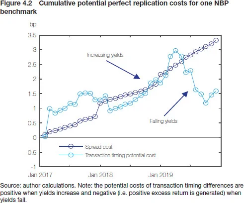
Thus, a portfolio manager striving to replicate, say, the US Treasury benchmark on a bond-by-bond basis would have faced the choice of either changing their positions or effectively taking on a small interest rate exposure vis-à-vis the benchmark. In the first case, their position may bleed due to risk misalignment, and in the other due to transaction costs that will typically not be borne by the benchmark. Indeed, in most cases, bond index benchmarks adjust positions at the market “mid” prices, whereas traders buy at the “offer” and sell at the “bid” side of the quotes (we will henceforth refer to this difference as the “spread cost”.)
Moreover, all benchmark “transactions” are recorded all at once at the end-of-day market close prices, whereas traders will execute throughout the day, or perhaps even over several days, leading to another source of mismatch in final performance. This factor may either act against or in favour of the managers (when rebalancing, they essentially buy duration and are thus exposed to yield changes), and its influence on portfolio returns can be surprisingly large in periods of increased market volatility (see Figures 4.1 and 4.2).55 A precise estimate of this effect would require an assumption on the timing of individual transactions and data on intraday securities prices. A simpler and quite effective alternative, which we used, is to assume that all rebalancing transactions are made at the beginning of the day – ie, at previous end-of-day prices. As a pointer, Box 4.3 discusses the effect on the rebalancing process of the initial impact of the coronavirus.
Box 4.3 Impact of March 2020 market turmoil on the rebalancing process
In early March 2020, the SARS-CoV-2 coronavirus, until then present in only a handful of countries, began to spread rapidly. Over the course of the next weeks, large numbers of infections were detected first in Western Europe and then in the United States, prompting local governments to adopt strict quarantine and social isolation measures that effectively shut down entire sectors of their economies. Financial markets reacted with a flight to quality. Risky assets such as equities and corporate bonds faced a severe sell-off while the safe haven assets rallied, with the yield of long-term government bonds falling to all-time lows. However, as the crisis deepened even the Treasury market began to feel the strain. At the short end of the curve, the yield of cash-equivalent Bills dropped below zero, whereas in the long end scarce liquidity actually drove the yields higher. Only once an extensive suite of emergency measures was introduced by the Federal Reserve did the situation abate, and markets regain their stability in the final days of March.
As the month drew to a close it became apparent that the low liquidity and increased volatility could generate unnecessary additional costs for benchmark-tracking investors during the upcoming March/April rebalancing. In recognition of the problem, the major providers (S&P Dow Jones, FTSE Russell and ICE Data Services) announced that their main indices would not be rebalanced, keeping the weights of individual constituents unchanged. Rebalancing was expected to resume at the end of April. The NBP Financial Risk Management Department decided likewise, and did not rebalance its benchmark portfolios at the beginning of April.

Lastly, over and above transactions related to rebalancing, portfolio managers also have to cope with coupon payments (which would need to be reinvested proportionally in benchmark bonds) and – specifically among central banks acting as agents for their national treasuries – cash inflows/outflows related to managing government accounts. The size of such cash flow fluctuations and the resulting forced portfolio adjustments can be considerable, driven by servicing foreign currency denominated government debt and other obligations, payments related to foreign trade, conversion of EU cohesion funds, etc.66 For example, the cumulative (net) inflow of EU funds into Poland since 2004 has exceeded €100 billion. A significant part of these inflows has been converted into Polish zloty by the NBP, increasing its foreign currency resources, triggering portfolio adjustments for reserve managers. Substantial flows can also occur if a central bank maintains a fixed currency structure of its portfolio and is forced to divest from a portfolio denominated in an appreciating currency while increasing the size of other portfolios.77 The daily scale of cash flows in and out of the NBP’s largest investment portfolios averaged 0.3–0.6% of their market values (2016–19). In comparison, the standard deviation of those portfolios’ daily return ranged from 0.05% to 0.11%.
Exactly how big such uncompensated transaction costs are will depend inter alia on the specific nature of the benchmark and the replication strategy followed, but they can constitute a non-negligible share of reserve manager’s excess returns. To appreciate this, note that for passive managers benchmarked to the Barclays High Yield Index, the performance drag related to such uncompensated transaction costs runs as high as 7.2bp for a dollar-based strategy and 12.4bp per month when hedging back into euros88 Bruce Phelps, and Ariel Edelstein, “Manager Performance Drag from Uncompensated Transaction Costs,” Barclays Capital Quantitative Portfolio Strategy (17 February 2012). – ie, well within the range of standard annualised excess return of Eurosystem dollar portfolio managers. Of course, the scale of uncompensated transaction costs is so large for the high-yield index mainly due to the low liquidity and wide bid/ask spreads in the corporate bond market, whereas the situation in high-grade, government-bond based benchmarks – where central bank reserve managers typically reside – is likely to look much better.
Still, it is not unreasonable to expect that such and similar effects could lead to an erosion of reserve managers’ excess returns, causing them to underperform their benchmarks despite taking little or no risk. Thus, it is perhaps worthwhile to consider how one might go about building and maintaining a replicating portfolio in the most cost-effective way, and related to that – against what “ideal standard” should efficiency of benchmark replication be judged/ assessed?
Bond index replication 101
As hinted above, there are two general approaches to replication: (i) bond-by-bond replication based on matching exactly individual benchmark positions; and (ii) replication based on matching the benchmark’s risk exposures, and possibly also selected other characteristics. While bond-by-bond replication might seem a straightforward and extremely effective approach to portfolio construction – as it does not rely on any sophisticated quantitative analysis and simply ensures that one has zero deviation versus the benchmark – we shall see below that it does not necessarily guarantee superior performance, with excess return depressed by uncompensated transaction costs. Moreover, exact position-based replication may not be practical, or even feasible, for some benchmarks. After all, strategic benchmarks – which by definition aim to represent as accurately as possible a given market segment – may easily be comprised of hundreds or even thousands of securities (see Table 4.1), some of which could be difficult or expensive to acquire, and once acquired to buy/ sell in line with subsequent rebalancing.
The alternative approach is based on the observation that being neutral with respect to a benchmark – ie, delivering consistently zero expected excess return – need not necessarily entail holding exactly the same positions as the benchmark, but rather holding the same risk exposures, which can often be achieved with much fewer instruments. For example, if we believed that the entire volatility of returns of the ICE US Treasury Master Index with around 260 bonds could be captured by its modified duration of around 6.8 (certainly a tall order), then – in principle – we might be happy replicating the entire index benchmark with just one or two bonds!
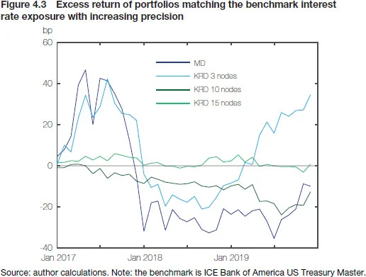
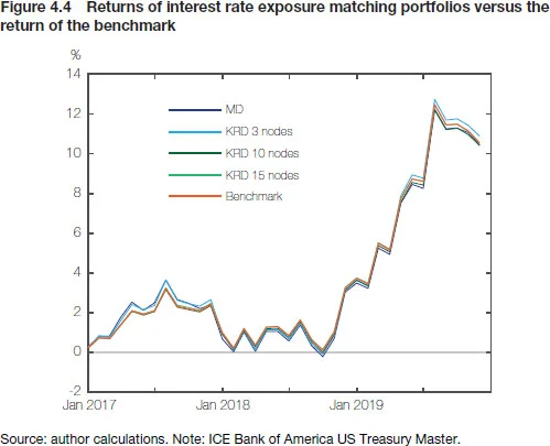
Clearly, portfolio-level modified duration (ie, a weighted average of durations of all bonds therein) captures only the first-order price effects due to parallel yield curve shifts. Hence, a more comprehensive representation of the benchmark’s risk profile will typically include also matching its overall convexity, sensitivity to selected key rates (ie, matching key rate durations) and possibly – depending on the benchmark – spread duration, as well as allocations to different countries, sectors or issuer groups. Figure 4.3 shows, for the Treasury Master Index, how tracking accuracy improves as we move from matching only modified duration to an increasing number of key rates: with 15 nodes, tracking difference falls to merely 2bp/month on average during the 36-month backtesting period. However, it is worth pointing out that even the crudest approach offers a return that, in a long-term perspective, is not materially different from the benchmark rate of return (see Figure 4.4).
From a mathematical standpoint, matching the risk exposure of a benchmark imposes a set of constraints on the proxy portfolio. Since the number of constraints will usually be much lower than the number of bonds in the benchmark, it follows that there can be many conceivable combinations of positions resulting in matched risk exposures. To choose the single best one requires setting up and solving an optimisation problem whereby one seeks to maximise a certain target variable subject to the set boundary conditions. If the target variable is a linear function of the benchmark, then the resulting problem can usually be solved very efficiently. For sufficiently small portfolios, this can even be done in Excel through its solver functionality (see Annex 4.1 on linear optimisation programming).
What could be some reasonable candidates for the target variables? In general, that will depend on the nature and composition of the strategic benchmark. For reasonably homogeneous benchmarks – eg, made up of single government bonds denominated in the local currency – a straightforward choice would be to maximise portfolio yield to maturity. Another potential candidate – especially for corporate bonds – would be the credit spread.
Certainly, a leaner portfolio containing only the relatively high-yield or high-spread bonds from the benchmark set might be desirable, although one should be careful not to overdo it by producing a portfolio that is, in a sense, too good to be true. Our conversations with portfolio managers suggest that such highly attractive securities may – rather unsurprisingly – be in high demand and thus difficult to purchase, which could be a problem if the number of securities in the optimised portfolio is relatively small to begin with. A remedy for some of these problems would be to focus instead on maximising some liquidity proxy – for instance, selecting bonds with highest amount issued, tight bid/ask spreads, youngest age (ie, shortest time since issuance) or highest liquidity score, capturing all these factors (and potentially others as well) simultaneously.
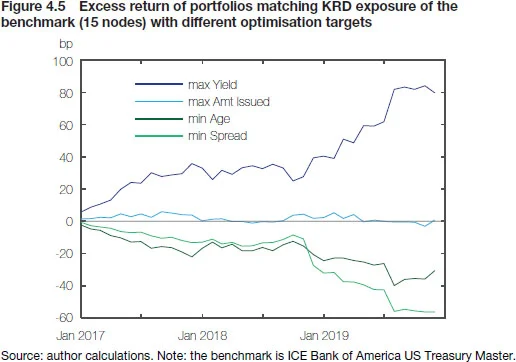
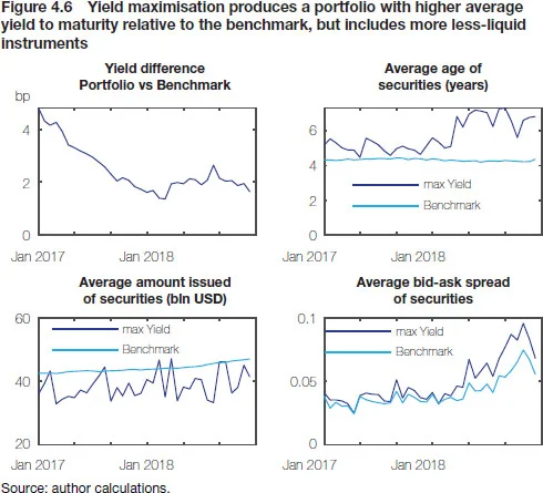
Again, which approach works best is an empirical matter, but the bottom line is that although the matching of risk exposures will in general not be perfect and is likely to leave portfolio managers with some residual uncertainty, it might save transaction costs and perhaps even generate a small return pickup if one is smart or lucky (or both!) with the choice of portfolio constituents. Consider the example in Figure 4.5, which shows for the US Treasury Master Index the monthly tracking errors of four replicating portfolios with different optimisation targets constructed according to the method outlined in Annex 4.1. Over our historical backtesting period, targeting yield would have produced truly spectacular results, with a consistently positive excess return of 2bp/month on average, leading to a cumulative return of about 80bp above the benchmark index. And while the original index comprises 260 bonds, the number of bonds in each of the replicating portfolios was only 16. However, given that higher return comes from selecting bonds with higher yields (the spread between the portfolio and the benchmark averaged 2.5bp), the portfolio also tends to be made up of less-liquid securities that might prove challenging to acquire in practice (see Figure 4.6 above).
Some practical considerations
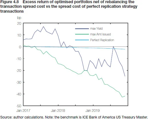
The lower liquidity of yield-maximising replicating portfolios is not the only problem, however. First, the leanness of the replicating portfolios also makes them very concentrated – with “optimal” position in some issues ranging as high as 25% – so that reserve managers with more sizeable reserves would struggle to operationalise such strategies. Second, there is a problem of portfolio turnover, as shown in Figure 4.7 for the entire backtesting exercise on a month-by-month basis. It seems that consistently maintaining the yield pickup while ensuring matched key rate duration (KRD) positions requires turning over upwards of 60% of portfolio market value at each rebalancing – on average 34 times as much as in the straightforward case of bond-for-bond replication. The estimated costs of such transactions would easily outgrow any excess return built up by carefully selecting the higher yielding bonds.
Unfortunately, this remains true even if the replicating portfolio is optimised to contain only the most-liquid issues. Again, the scale of transactions needed to maintain neutrality after each rebalancing eats away the excess return, leading to serious benchmark underperformance relative to the simple strategy of perfect position replication. While it is clear that the latter also suffers from uncompensated transaction costs, it is certainly superior to the optimised alternatives, neither of which can be readily implemented anyway given the concentration problem mentioned above.
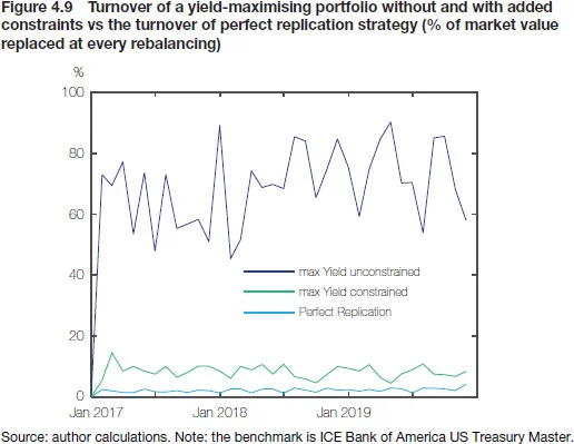
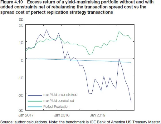
However, optimisation has more to offer than we have given it credit for so far. The basic set-up of matching KRDs can be easily extended by adding more boundary conditions to address both turnover and position concentration. We do just that in Figures 4.9 and 4.10 (below), which again show the backtesting results for a portfolio optimised to match KRD exposures of the US Treasury Master Index with high-yield benchmark Treasury bonds, but constrained in two ways:99 See Annex 4.1 for the details of implementing the constraints. (i) to rebalance with as little turnover as possible; and (ii) to prohibit positions larger than 2% for an individual issue. The collapse in rebalancing-induced turnover is spectacular, as the volumes traded come close to the perfect bond-by-bond replication (which needs little maintenance owing to the relatively long duration of the benchmark). As a result, bond selection works its magic and the yield pickup eventually leads to a decent-sized excess return – after transaction spread costs – of around 10bp over the entire 36-month period. The replicating portfolio is not as lean as before – with up to 113 issues sampled from the benchmark index, consisting of around 260 instruments – but as a result it should at least be implementable in practice.

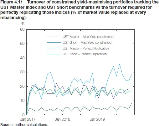
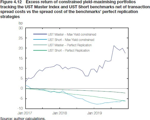
Unfortunately, the potential to generate cost-adjusted excess returns through yield maximisation and turnover constraints depends to a certain degree on the characteristics of the benchmark we are trying to replicate. To see this, consider a markedly shorter benchmark, which we will refer to as UST Short, with an overall modified duration of 1.0, about 145 issues and roughly two-thirds of its composition made up by securities with residual maturities of below one year. Compared to the broad US Treasury Master Index – whose modified duration averaged 6.4 and number of issues stood at 260 – our new short benchmark will generate considerably larger turnover upon each rebalancing (amounting to about 13% of its market value), which in turn translates into substantial uncompensated transaction costs upwards of 2bp/ year versus 0.70–0.80bp/year for the Treasury Master Index (see Figure 4.11). With such a short-duration benchmark, our previous technique of limiting turnover and selecting high-yield securities from the benchmark will not necessarily guarantee superior results relative to bond-by-bond replication (Figure 4.12). After all, we now have fewer instruments to choose from (with correspondingly lower yield dispersion) and greater turnover stemming from the short maturities of benchmark issues. Thus, to deal with a huge turnover that is likely to be characteristic of the short-duration benchmarks preferred by central bank reserve managers, we need a smarter and more refined approach.
Introducing derivatives
A recurring theme of this chapter is that what needs to be taken into account in evaluating various replicating strategies is the level of uncompensated transaction costs – ie, costs borne by portfolio managers but not reflected in the benchmark. The bulk of such uncompensated costs arises in the process of rebalancing, eg, when short-maturity securities are simply removed from the index (to maintain its duration), prompting sales by managers replicating the benchmark on a bond-by-bond basis. Specifically, with monthly rebalancing usually it is securities with less than one month to maturity that are removed, whereby the share of such securities – and the associated cost burden – is of course likely to be higher the shorter the duration of the benchmark.
This suggests yet another refinement to our replication approach: if it is the forced selling of short residual maturity securities that generates significant turnover and uncompensated costs, then why not simply allow these securities to mature while managing the resulting duration exposure with the use of Treasury futures. At maturity, the redemption proceeds will need to be reinvested, which can be done in a way that restores the KRD exposure of the portfolio to that of the benchmark. This leads to an observation that if we are able to effectively hedge the KRD exposure with futures, then all rebalancing transactions can be done as a side effect of such reinvestments, entirely independent of the benchmark-rebalancing schedule. The main benefit of such an approach is that even if it does not reduce the overall turnover, it replaces a significant amount of sales, which generate spread cost, with redemptions.
Specifically, we can consider the following replication strategy for a US Treasury benchmark that consists of securities with maturity of up to ten years but has a relatively short modified duration of 1.8 achieved by heavily overweighting the front end of the yield curve (60% allocated to securities maturing in less than one year).
-
-
We start by assembling a portfolio that perfectly replicates the benchmark.1010 We chose not to start with an already optimised portfolio so that we could simulate the situation of a portfolio manager who decides to abandon the strategy of perfect replication.
-
-
-
We monitor both the benchmark and the actual portfolio daily.
-
-
-
We abstain from any actual securities transactions when the benchmark is rebalanced at the end of each month, and use a daily adjusted portfolio of Treasury futures contracts1111 For reference, we have used the following contracts: TU for 2Y, FV for 5Y, TY for 7Y and UXY for 10Y. to offset the resulting KRD exposure.
-
-
-
When a security matures in the portfolio, we rebalance through a linear yield-maximising optimisation (see Annex 4.1) and close out the futures position. The optimisation is constrained to minimise the resulting turnover and prohibit positions of over 5% in any security.1212 We also introduce a restriction that limits the instruments that can be bought at rebalancing to those maturing in at least one month in order to further reduce the amount of turnover.
-
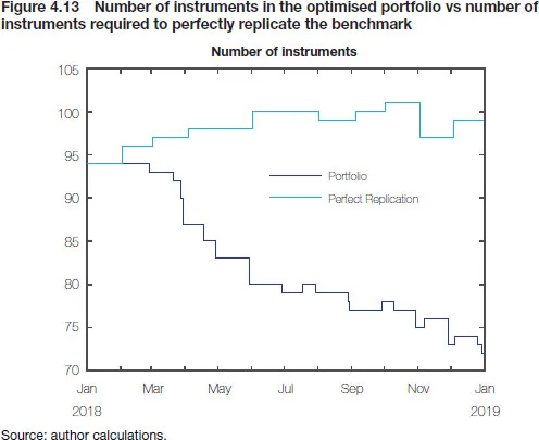
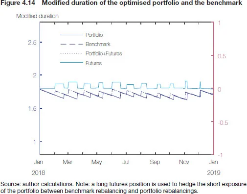
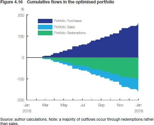
The mechanics of the approach is shown in Figures 4.13 and 4.14. Both portfolios start with 94 securities, but over the 12 months included in the backtesting exercise the composition of the proxy portfolio visibly deviates from the benchmark. The subsequent optimisations lead to a portfolio of 75–80 instruments as opposed to about 100 in the benchmark. We can also see how occasional KRD exposure arising from “ignoring” benchmark rebalancing is neutralised by means of a long futures position, closed out once redemptions allow for physical portfolio adjustment. Figures 4.15 and 4.16 provide an overview of the size of purchases, sales and redemptions in the perfect replication and optimised portfolios. The overall scale of turnover in both portfolios is similar and considerable, which comes as no surprise given the short-term structure of the benchmark. However, in the optimised portfolio securities are removed primarily by allowing them to mature rather than by means of market sales, which significantly reduces the spread costs. Note also that changes to portfolio composition are smaller and more frequent than in the case of bond-for-bond replication, which might actually be favourable from a liquidity or operational perspective.

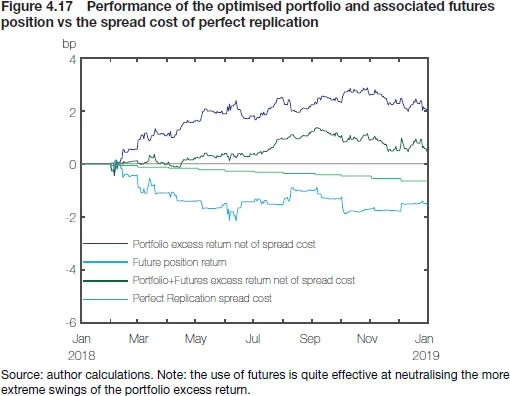
Ultimately, the proof of the pudding is in the eating, so Figures 4.17 and 4.18 focus on the backtested performance of that strategy. Over the course of the backtesting period, yields were moving higher so occasional short-duration positions relative to the benchmark generated an additional positive return for the securities portfolio. Using futures to close the duration gap neutralised this effect, which can be seen especially well in the initial months when the composition of the portfolio had not yet deviated from that of the benchmark. In the following months through the course of subsequent optimisations, the portfolio started to generate an excess return due to selection effects, which was unaffected by the futures position. The strategy of rebalancing as a side effect of redemptions successfully limited the spread cost associated with yield maximisation so that, at the end of the year, the overall excess return of our strategy remained positive even net of transaction spread cost.
The simulations show that a simple rule-based strategy is able to accurately track the benchmark return, and if well-designed may even generate a positive excess return. The outperformance, while certainly a welcome result, should not overshadow what we believe is the main finding of the exercise, namely that replicating the risk exposure of a benchmark can produce portfolios where returns do not deviate excessively from that of the benchmark. Another way of expressing this is that maintaining a neutral position relative to the benchmark should not, except in extreme cases, be understood as the replication of the position of each and every instrument in the benchmark. While this observation may come as natural for a typical active manager, its implications could be of importance for central banks, which are particularly risk-averse and often follow benchmarks that are simple enough to make perfect replication strategies seem both practical and attractive.
In reality, attempting a perfect replication in the presence of market bid/ask spread and without consideration of the timing of individual transactions, for a fixed income index is most often inefficient. Note that, in the simulations we adopted a most conservative estimate of the costs, whereas a real-life portfolio manager could face different, perhaps worse, prices and duration exposure due to differences in timing. The simulated portfolio did not have to accommodate any external inflows or outflows, which would make perfect replication much more difficult to follow. At the same time, it is not unreasonable to assume that portfolio managers working full time, and having a good picture of the markets would be able to construct much more efficient risk exposure matching portfolios than those set by our simple rule-based approach.

Conclusions
The practical challenges of effective benchmark replication, often treated as little more than a side note to the major issue of strategic allocation and benchmark selection, have so far received limited attention. While it is true that those challenges are often idiosyncratic and specific to particular institutions, there is no doubt that an analytical treatment could provide suggestions and solutions that could be of use in day-to-day asset management operations. In this chapter, we looked at the issue of benchmark replication from the point of view of a central bank investing in government bond markets. Central banks, being public risk-averse institutions, often pursue essentially passive strategies even if their portfolio managers are allowed to take active positions. Such circumstances, and increased scrutiny of central banks’ financial results, can make the issue of replication efficiency one of major concern.
Our approach makes use of a simple quantitative framework that provides estimates of risks and returns associated with different replication strategies. Specifically, we show that following a simple rule-based risk-exposure replication allows the portfolio to track the benchmark with acceptable accuracy while also allowing space for active management via issue selection, and that using futures contracts to manage duration exposure can provide even greater flexibility. It should be noted, however, that although the main findings are applicable to most benchmarks, there is no “one-size-fits-all” solution, and particularities of replication will differ depending on the structure and duration of a given benchmark.
That said, our analysis confirms that even conservative portfolio managers should not consider themselves prisoners of their benchmarks since they should be able to effectively track their performance by using portfolios that consist of different instruments. This is not without consequence for strategic allocation decisions as well since it should free those responsible for setting the benchmarks from the responsibility to ensure that the selected indices are perfectly replicable.
The views expressed are those of the authors and do not represent the official position of the NBP.
Annex 4.1 Optimisation
To find the composition of portfolios that match the risk exposure of a given benchmark, we used a straightforward linear programming approach. The most basic form of our problem is to devise a vector of weights wP of available instruments so that the KRD exposure of the resulting portfolio matches that of the benchmark, ie:
KRDT wP = KRDT wB
where wB are benchmark instrument weights and KRD is the matrix of KRD exposures for individual securities. Naturally, the weights wP need to sum up to 1, and since we exclude short positions and leverage all elements of wP ∈ [0,1]. For the optimisation to the work, we also require the objective function, which in our case may maximise the yield of the portfolio or some measure of its liquidity.
As discussed, the basic approach produces well-functioning portfolios but is of little practical value since the optimal portfolio in a given month may consist of entirely different securities than in the previous month, which would require unrealistic amounts of turnover on rebalancing days. To mitigate this problem, we need to take into account not only the current composition of the benchmark but also the composition of the portfolio before rebalancing. The subject of optimisation will then be not the absolute weights of instruments but the changes in weights relative to the initial composition of the benchmark, which will allow us to impose a constraint on the sum of these changes (ie, on the turnover). In addition, a point can be made that since we require a precise equivalence of portfolio and benchmark KRD exposures, a substantial portion of turnover is generated by relatively modest KRD adjustments, which can be particularly true for short-term instruments. Therefore, if we let the shorter KRD exposure (eg, six months) deviate slightly from that of the benchmark, we might be able to further reduce the turnover while introducing only very limited interest risk exposure.
Another potentially problematic result is a low number of securities used in the portfolios. In general, for n KRD nodes a basic optimised portfolio will contain at most n+1 instruments, some with weights up to 25%. Such a concentration may not be of great concern for small portfolios, but for large ones the required investment might simply be unfeasible. An obvious solution is to introduce a constraint on the weights of individual securities.
The complete form of our optimisation problem, which includes the extensions discussed above, is as follows. Let x = [ps ] be a vector of length 2n, where n is the number of available instruments. The first half of values in x, designated as p, contains weights of individual instruments that are purchased, while the second half, s, contains weights that are sold. Let w0 be initial weights in the portfolio (before rebalancing) while w1 are final weights, so that w0 + p – s = w1. Finally, as before, let wb be weights of instruments in the current benchmark (after rebalancing) and KRD a matrix of key rate durations for individual securities. Our optimisation problem is to find x, which maximises or minimises the objective function – eg, max yTx, where y are the yields of individual instruments subject to the following constraints:
where c is a vector specifying how much each of the portfolio’s KRD exposures is allowed to deviate from the benchmark, tmax is a limit on turnover (ie, p + s) and smax is the maximum allowed weight for any instrument. The first of the constraints is responsible for keeping the portfolio KRD exposure within the specified deviations around the benchmark exposure while limiting the turnover. The second constraint ensures that the value of purchases equals the value of sales, so that ∑w1 = ∑w0 = 1. The final constraint prohibits purchases that would increase the weights above smax and limits sales to exclude the possibility of negative weights.
To find x that satisfies our rebalancing objectives with the least turnover, we apply the optimisation iteratively, starting with tmax = 0.01 and increasing it by 0.01 until a solution is found.
Only users who have a paid subscription or are part of a corporate subscription are able to print or copy content.
To access these options, along with all other subscription benefits, please contact info@centralbanking.com or view our subscription options here: subscriptions.centralbanking.com/subscribe
You are currently unable to print this content. Please contact info@centralbanking.com to find out more.
You are currently unable to copy this content. Please contact info@centralbanking.com to find out more.
Copyright Infopro Digital Limited. All rights reserved.
As outlined in our terms and conditions, https://www.infopro-digital.com/terms-and-conditions/subscriptions/ (point 2.4), printing is limited to a single copy.
If you would like to purchase additional rights please email info@centralbanking.com test test test
Copyright Infopro Digital Limited. All rights reserved.
You may share this content using our article tools. As outlined in our terms and conditions, https://www.infopro-digital.com/terms-and-conditions/subscriptions/ (clause 2.4), an Authorised User may only make one copy of the materials for their own personal use. You must also comply with the restrictions in clause 2.5.
If you would like to purchase additional rights please email info@centralbanking.com test test test


