Assessing sources of excess return: style analysis for active investing
Eduardo Hoyos Castro, Fernando Torres and Carlos Alvarez
Trends in reserve management: 2018 survey results
Denmark’s move to a holistic and dynamic risk budget
Custody in 2025: a primer for reserve managers
Assessing sources of excess return: style analysis for active investing
The role of reserves in Iceland’s post-crisis recovery
Interview: Solomon Kavuma
For an institutional investor it is very important to understand the sources of the excess return generated by both its external and internal asset managers. Certainly, not all excess returns are produced equal – for instance, an asset manager may be very skillful at generating excess returns by timing the market, while another may generate excess returns by having a levered buy- and-hold exposure to a particular asset class. In this sense, the first manager may be generating pure alpha, whereas the second is simply delivering a levered beta. An understanding of the different styles within the portfolio allows institutional investors to recognise the roles of various managers in terms of the expected active risk and returns, and may provide relevant information to be considered when evaluating the benchmark. This is also relevant for central banks. Indeed, with an increasing focus on returns at a time of low yields, central banks have looked to diversify, notably in equity markets, often making use of external managers.
For official institutions, central banks, and asset managers in general, it is important to have periods of review of current benchmarks and current asset managers to ensure the portfolios are aligned to the investment objective. In our case, as part of this process we wanted to evaluate the internal and external portfolio managers, as well as to develop an assessment methodology that went beyond the usual risk-adjusted return.
In this chapter, we aim to explain the excess returns of a set of managers as a function of different investment strategies or “market factors”, with the unexplained component representing the skill of the manager. We prefer to explain the excess returns in terms of factors rather than asset classes as the return of an asset class may be related to more than one factor. In addition, as will be seen, our approach is relatively simple and allows an official institution or central bank to perform its own performance analysis without the need for sophisticated software. The chapter is divided in three sections: a definition of the model, a case study, and a summary of conclusions.
Model definition
A financial institution should have an objective evaluation process for its asset managers, one that is able to provide qualitative and quantitative performance measures as reliable inputs for decision-making. For example, if an institution wants to compare active management between two or more portfolio managers, and answer questions such as “is their alpha ‘pure skill’ or is it more like ‘smart’ beta”?
In the process of evaluating the performance attribution of different managers, we try to classify them according to their ability to generate excess returns in ways that are specific to each manager. In this regard, the style and skill decomposition single-factor model developed by Jensen11Michael C. Jensen, “The Performance of Mutual Funds in the Period 1945–1964,” Journal of Finance 23 (1968): 389–416. gives us some insights:
where the portfolio return (Rt) is regressed on a risk asset, whether the index or market return (Rmt) and the risk-free return (Rft).
In our analysis, we express the excess returns as a one-factor model:
Since the risk-free asset, which has a low variability, could skew the results, we eliminate that term; therefore, the previous relationship can be expressed as:
In this approach, the return is generated in two ways. The first is the proportion of the risk asset in the portfolio, which is classified as style:
Since we are not considering the risk-free asset, we have that:
Second, there is the idiosyncratic ability of the manager to generate returns, which is classified as skill:
This idea can be generalized if one considers that the portfolio return depends on more than one factor. The Arbitrage Pricing Theory developed by Stephen Ross in 1976, or APT, provides a framework for the multifactorial model. This model considers that the return of a portfolio can be explained by a weighted sum of the return of a number of factors and the return of the riskless asset:
In this manner we can define style return as the fraction of the total return that is explained by the factors, and the skill return as the remainder portion. In the finance literature, skill has usually related to security selection. However, for the purpose of this analysis we will assume it includes dynamic trading strategies (where exposures can change frequently). This assumption makes sense since correlation between an asset’s return and a dynamic trading strategy in the asset is small, or there may even be no correlation at all.
In our analysis below, we attempt to evaluate and rank four managers and their ability to generate returns in excess of their benchmark index. As this is a case with multiple-factor portfolios and benchmark indexes, to give some insight we took into consideration the extreme cases for the regressions.
Case 1: Pure style-driven returns
For this case, there could be a scenario where there are positive excess returns of a manager’s portfolio that is highly correlated with market-factor returns, and there is small (or no proportion at all) of the excess returns that are not explained by market factors. In this case, the regression of the portfolio excess returns on the factor returns would show no significance of the intercept (small t-statistic), but rather that the model market factors as a whole are significant (small F-test); it would also show that individually all market factors are significant in the model and, finally, the model would fit well with the data of returns (R-squared close to 1).
In this case, the manager’s excess return is pure style return, and is related to the way they allocated its positions in the market factors. Therefore, it would also be safe to assume that the manager does not use (or uses very little) dynamic trading strategies.
Case 2: Pure skill-driven returns
The other extreme scenario would be positive excess returns in the manager’s portfolio, but with no correlation at all with the market-factors returns. Therefore, the excess return is not explained by the market-factors returns. In this case, the regression of the portfolio excess return on the factor returns may show a high significance or some significance of the intercept, the model market factors as a whole have little or no significance, and also individually few or no market factors at all are significant.
The model would not fit well with the data of the returns. In this case, the manager’s excess return is skill return, and is related to the returns of the specific securities selected by the manager and the returns of the dynamic trading strategies used by them. Note that the opposite extreme scenarios are also plausible and follow the same principle, so we can classify negative excess returns as negative style or negative skill returns.
The approach of this chapter is based on a multi-factor model. If we extend the single-factor to a multi-factor model, we get:
Therefore, we now have put in place the building blocks for our analysis, with linear regressions and the criteria for mapping managers along the line between pure skill and pure style. We are set to apply this to our particular case, and see whether the managers of our portfolios can be classified and ranked according to the way in which they generate excess returns.
Case study
The main objective of this chapter is to determine the level of style (or skill) management of four asset managers by means of statistical methods. The first two portfolios are managed externally and share the same benchmark, the third portfolio is managed internally, and the fourth is managed by three different managers and has a benchmark that includes all the indexes in the other benchmarks.
| Portfolio | BMK 1: 31 December 2012 to 31 January 2015 | BMK 2: 31 January 2015 to 31 August 2016 |
| Portfolio 1 and 2 | 50% money market, 16.7% six- month T-bills and 33.3% TIPS 1–10 years | 80% money market and 20% six-month T-bills |
| Portfolio 3 | 75% money market and 25% six-month T-bills | 80% Treasuries 0–1 years, 10% Treasuries 0–5 years and 10% TIPS 1–10 years |
| Portfolio 4 | 33% money market, 33% six-month T-bills and 33% TIPS 1–10 years | 40% money market, 40% Treasuries 0–1 years, 15% Treasuries 0–5 years and 5% TIPS 1–10 years |
| Source: authors. | ||
The whole observation period is from 31 December 2012 to 31 August 2016, but there is a change in the benchmark for the external managers and for the internally managed sub-portfolios starting from 31 January 2015. The benchmarks are set as shown in Table 4.1.
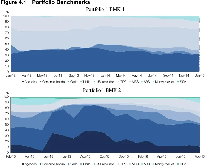
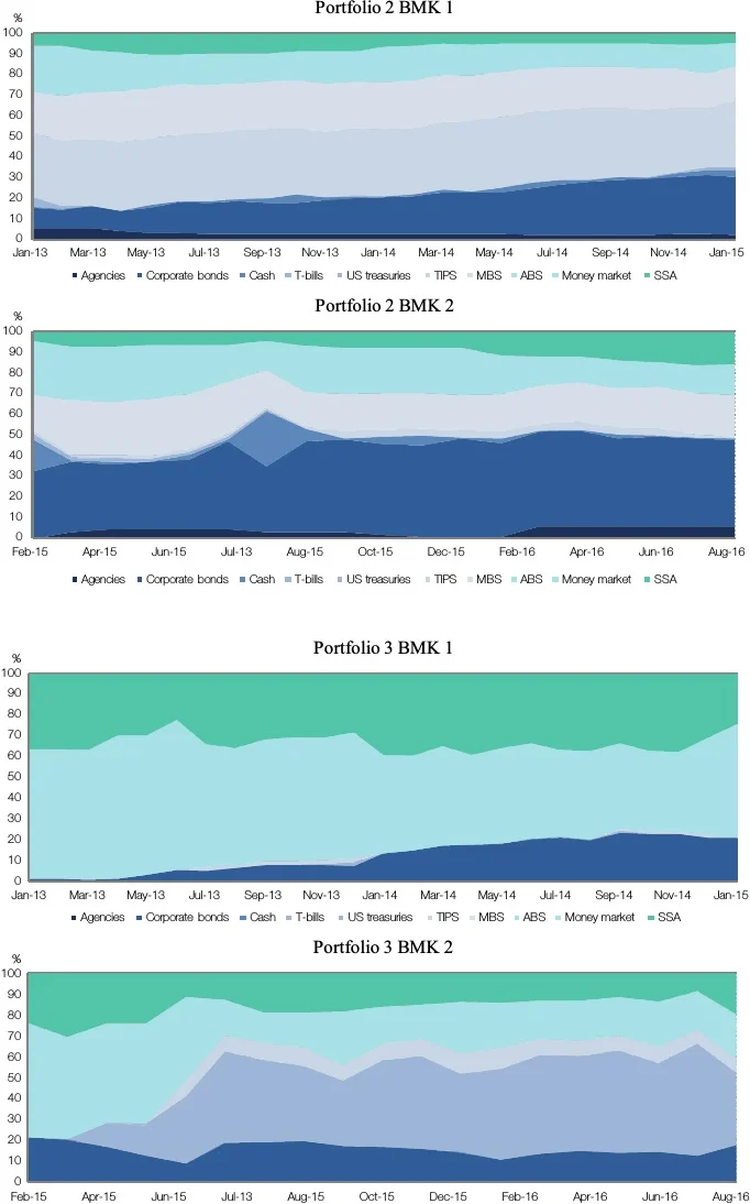
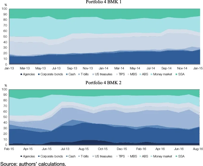
The allocations of the 4 portfolios throughout the benchmark periods are as above.
There is never a point in time where the currency exposition other than USD exceeds 1%, so the currency breakdown is not shown. Managers 1 and 2 are somehow active in currencies but with minimal amounts.
In the change of benchmark, portfolios 1 and 2 migrate from a portfolio with a significant duration exposure to a short-duration portfolio more focused on corporate spread factors and money market. In the case of portfolio 3, it changes from a short-duration money-market portfolio to a longer-duration portfolio that includes Treasury inflation-protected securities (TIPS). Finally, in the case of portfolio 4, it changes by reducing the overall duration and the exposure to TIPS, and by increasing the Treasuries’ exposure. The risk factors available for the managers’ strategies, and thus factors of the models, are shown in Table 4.2.
For the purpose of this analysis the risk factors are approximated as follow:
| Fixed income | Equity | Commodities | Currency |
| Duration (D1) | S&P500 | GSCI | Euro (€) |
| Slope (D2) | UK pound (GBP) | ||
| Break-even inflation (BEID1) | Japanese yen (¥) | ||
| Break-even inflation slope (BEID2) | Swiss franc (CHF) | ||
| Corporate bonds spread (CORPD1) | |||
| Corporate spread slope (CORP D2) | |||
| Mortgage-backed securities spread | (MBS) | ||
| Source: authors. | |||
-
-
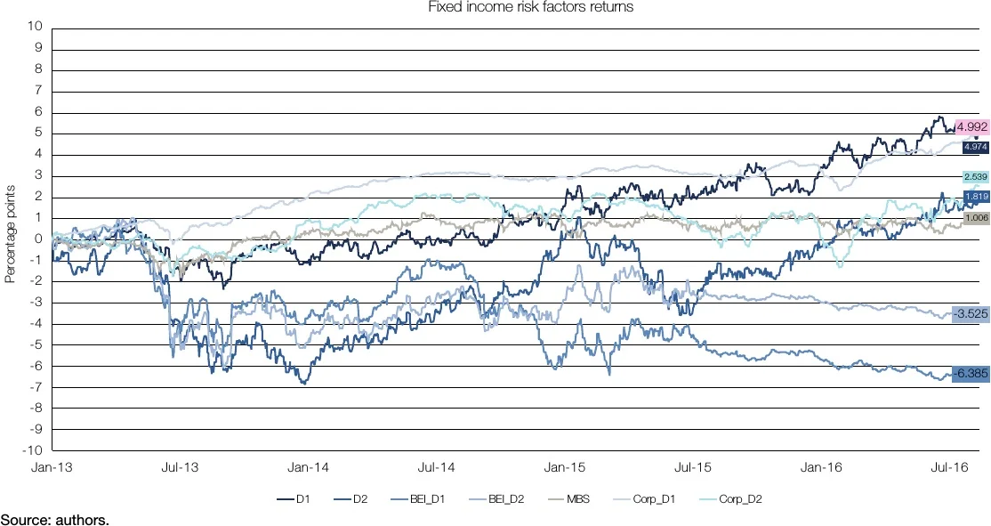
D1 is computed using the duration return of the 3 to 5 year Merrill Lynch US Treasury bond Index (G202) minus the 1 month Libor index return (LUS1).
-
-
-
Slope (D2) is computed using the duration adjusted return of the difference between the 7 to 10 year and the 1 to 3 year Merrill Lynch US Treasury bond Indexes (G402 and G102). The computation is made adjusting the weights so the duration of the long position in the 7 to 10 year index matches the duration in the 1 to 3 year index and the net duration of the position is zero.
-
-
-
Break Even Inflation (BEI D1) is computed using the excess return of the 3 to 5 year inflation linked index index(G2QI) versus treasuries of the 3 to 5 years Merrill Lynch US Inflation Index (G202).
-
-
-
BEI Slope (BEI D2) is computed using the difference of the duration adjusted excess returns of the 7 to 10 year and the 1 to 3 year Merrill Lynch US Inflation-Linked Treasury Indexes (G4QI and G1QI). Each index adjusted for duration by subtracting the equivalent US Treasury bond index (G402 and G102 respectively).
-
-
-
Corporate bond spread factor (CORPD1) is approximated with the excess returns versus treasuries of the Merrill Lynch 3 to 5 year A-AAA index (C210) duration adjusted.
-
-
-
Corporate spread slope return (CORPD2) is computed with the difference between the difference of the excess return versus treasuries of the Merrill Lynch 7 to 10 year A-AAA index (C410) duration adjusted, and the Merrill Lynch 1 to 3 year A-AAA index (C110) duration adjusted.
-
-
-
Mortgage Back securities return is approximated with the duration adjusted excess return versus treasuries of the Merrill Lynch M0A0 Index.
-
-
-
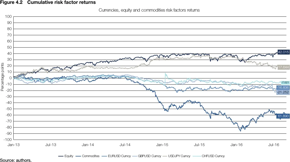
For equity, the analysis takes the return of the S&P 500 index, for commodities, the Goldman Sachs commodity index, and for currencies the analysis takes the return of the four major currencies.
-
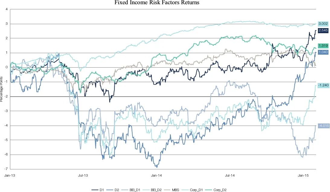
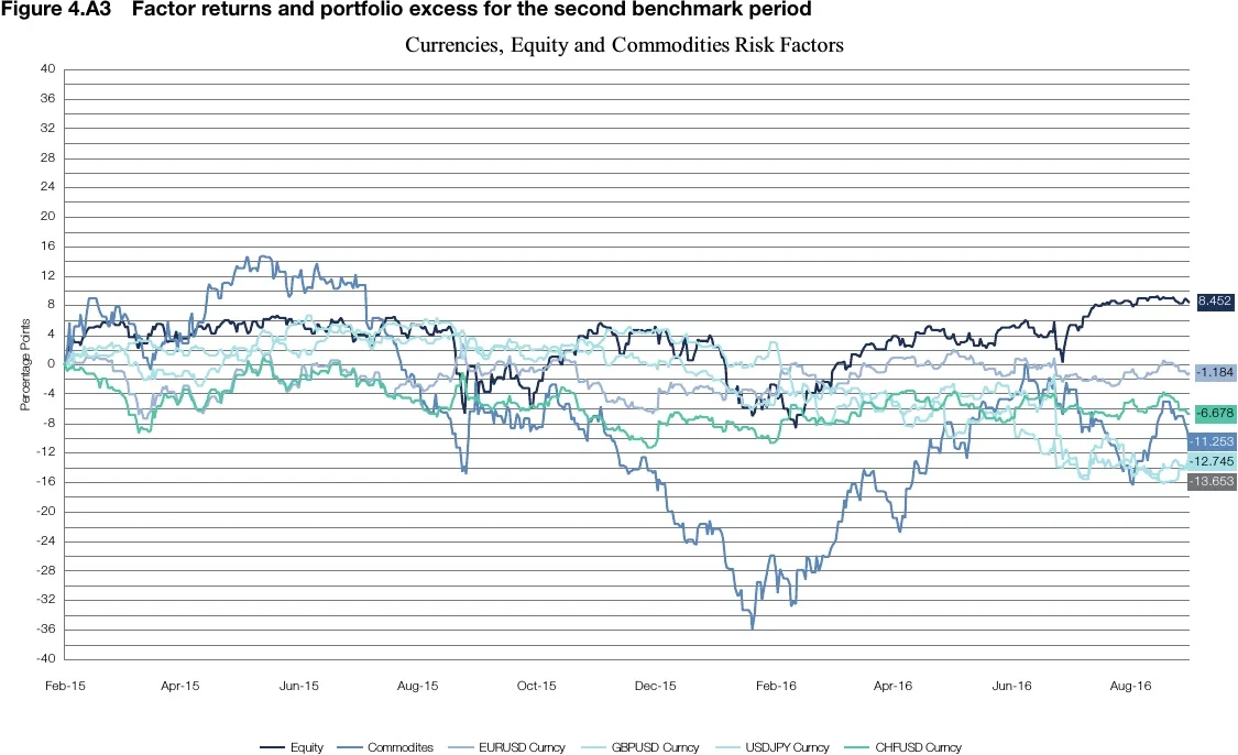
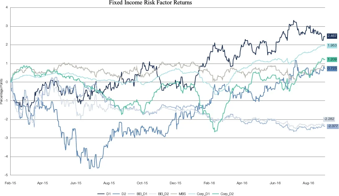
To get a preliminary idea of the behaviour of the risk factors, Figure 4.1 presents the cumulative returns of the risk factors for the whole period. For the different benchmark period graphs, see the Appendix to this chapter.
To illustrate how the analysis is performed, the results for the first portfolio will be broken down and analysed thoroughly, before a general analysis of the four portfolios is presented.
Portfolio 1 analysis
When analysing the first portfolio through the whole period, the results indicate, on the one hand, that as a set the factors selected are important, and given the p-value of the F-test, there is evidence that the model factors as a whole are relevant at any level of significance. On the other hand, the low R-squared indicates that the model does not fit well with the data.
| Model formula: ER ≈ β1D1 + β2D2 + β3BEID1 + β4BEID2 +β6MBS + β7CORPD1 + β8CORPD2 + β9Equity + β10Commodity + β11EUR + β12GBP + β13JPY | |||
| Coefficients | Estimate β | Pr (>|t|) | Signif. |
| Intercept | 0.011410 | 0.49710 | - |
| D1 | -0.057695 | 0.01923 | 0.050 |
| D2 | 0.001306 | 0.92588 | - |
| BEID1 | 0.056842 | 0.01948 | 0.050 |
| BEID2 | -0.093088 | 0.00201 | 0.010 |
| MBS | -0.024308 | 0.42373 | - |
| CORP D1 | 0.001644 | 0.98169 | - |
| CORP D2 | 0.094327 | 0.01570 | 0.050 |
| Equity | 0.001861 | 0.54590 | |
| Commodities | -0.000845 | 0.66585 | - |
| EUR | 0.004394 | 0.36119 | - |
| GBP | -0.002527 | 0.54441 | - |
| JPY | 0.004745 | 0.21805 | - |
| CHF | 0.001357 | 0.61884 | - |
| Residual Standard Error | 0.06059 | ||
| Multiple R- Squared | 0.06579 | ||
| F- Statistic | 7.178 | P-Value | 1.10E-13 |
| Source: authors. | |||
Table 4.3 shows that even if the factors as a whole are relevant in this analysis, most of the excess returns cannot be explained by the returns of the factors, and there are very few style-driven strategies. The individual factors identified as relevant are duration (D1), break-even inflation (BEID1), breakeven inflation slope (BEID2) and corporate spread slope (CORP D2). If the manager has style-driven strategies, it is more likely that they would relate to these factors. Since there is little statistical evidence of style-driven strategies, the conclusion in this case is that the likelihood of this manager being skill-strategy driven is high.
Now, for the period between 1 January 2013 and 31 January 2015, the benchmark for this portfolio was 50% money market, 16.7% six-month T-bills and 33.3% TIPS 1–10 years. These results are consistent with the whole period, and the F-test shows that at any level of significance the model is relevant. The R-squared indicates that the returns of these factors do not explain the majority of the data variance, giving no evidence of style-driven strategies. The individual factors that are identified as relevant are duration (D1) and break-even inflation (BEID1).
| Model formula: ER ≈ β1D1 + β2D2 + β3BEID1 + β4BEID2 +β6MBS + β7CORPD1 + β8CORPD2 + β9Equity + β10Commodity + β11EUR + β12GBP + β13JPY + β14CHF | |||
| Coefficients | Estimate β | Pr (>|t|) | Signif. |
| Intercept | 0.001391 | 0.63767 | - |
| D1 | -0.189003 | 0.00103 | 0.010 |
| D2 | 0.024243 | 0.36834 | - |
| BEID1 | 0.096399 | 0.02447 | 0.050 |
| BEID2 | -0.070773 | 0.14122 | - |
| MBS | -0.020021 | 0.67379 | - |
| CORP D1 | 0.020700 | 0.87872 | - |
| CORP D2 | 0.106445 | 0.14678 | - |
| Equity | 0.002126 | 0.72693 | - |
| Commodities | -0.002432 | 0.60953 | - |
| EUR | 0.007115 | 0.46771 | - |
| GBP | -0.001046 | 0.91804 | - |
| JPY | 0.004384 | 0.52803 | - |
| CHF | 0.002669 | 0.48683 | - |
| Residual Standard Error | 0.07941 | ||
| Multiple R- Squared | 0.07493 | ||
| F- Statistic | 4.661 | P-Value | 9.02E-08 |
| Source: authors. | |||
For the next period, between 31 January 2015 and 31 August 2016, the benchmark for this portfolio is 80% money market and 20% six-month T-bills.
| Model formula: ER ≈ β1D1 + β2D2 + β3BEID1 + β4BEID2 +β6MBS + β7CORPD1 + β8CORPD2 + β9Equity + β10Commodity + β11EUR + β12GBP + β13JPY + β14CHF | |||
| Coefficients | Estimate β | Pr (>|t|) | Signif. |
| Intercept | 0.00124 | 0.00342 | 0.010 |
| D1 | -0.01717 | 0.00249 | 0.010 |
| D2 | -0.01328 | 0.00013 | 0.001 |
| BEID1 | 0.01478 | 0.04178 | 0.050 |
| BEID2 | -0.03065 | 0.00012 | 0.001 |
| MBS | -0.00073 | 0.94635 | - |
| CORP D1 | 0.07358 | 0.00002 | 0.001 |
| CORP D2 | 0.04180 | 0.00001 | 0.001 |
| Equity | -0.00068 | 0.33364 | - |
| Commodities | 0.00029 | 0.46146 | - |
| EUR | -0.00069 | 0.64249 | - |
| GBP | 0.00009 | 0.91805 | - |
| JPY | 0.00263 | 0.00789 | 0.010 |
| CHF | -0.00019 | 0.89621 | - |
| Residual Standard Error | 0.009984 | ||
| Multiple R- Squared | 0.477 | ||
| F- Statistic | 39.49 | P-Value | 2.20E-16 |
| Source: authors. | |||
The results in this period contrast sharply with the whole period and those of the first period. Since the F-test indicates that at any level of significance the model factors as a whole are relevant, and the R-squared indicates that with the returns of these factors you can explain at least 47% of the returns of the portfolio so the model to some degree fits the data, there is evidence of style-driven strategies. The individual factors that are identified as relevant are duration (D1), slope (D2), break-even inflation (BEID1), break-even inflation slope (BEID2), corporate spread (CORPD1), corporate spread slope (CORP D2) and Swiss franc Swfr.
Four portfolios: general analysis
Having analysed each portfolio, we now carry out a general analysis of the four portfolios to classify and rank them according to investor preferences. Table 4.6 shows the results for the remaining portfolios.
| Model formula: ER ≈ β1D1 + β2D2 + β3BEID1 + β4BEID2 +β6MBS + β7CORPD1 + β8CORPD2 + β9Equity + β10Commodity + β11EUR + β12GBP + β13JPY | |||
| Portfolio 1 | |||
| Coefficients | Estimate β | Pr (>|t|) | Signif. |
| Intercept | 0.011410 | 0.49710 | - |
| D1 | -0.057695 | 0.01923 | 0.050 |
| D2 | 0.001306 | 0.92588 | - |
| BEID1 | 0.056842 | 0.01948 | 0.050 |
| BEID2 | -0.093088 | 0.00201 | 0.010 |
| MBS | -0.024308 | 0.42373 | - |
| CORP D1 | 0.001644 | 0.98169 | - |
| CORP D2 | 0.094327 | 0.01570 | 0.050 |
| Equity | 0.001861 | 0.54590 | |
| Commodities | -0.000845 | 0.66585 | - |
| EUR | 0.004394 | 0.36119 | - |
| GBP | -0.002527 | 0.54441 | - |
| JPY | 0.004745 | 0.21805 | - |
| CHF | 0.001357 | 0.61884 | - |
| Residual Standard Error | 0.06059 | ||
| Multiple R- Squared | 0.06579 | ||
| F- Statistic | 7.178 | P-Value | 1.10E-13 |
| Portfolio 2 | |||
| Coefficients | Estimate β | Pr (>|t|) | Signif. |
| Intercept | 0.00123 | 0.00431 | 0.010 |
| D1 | -0.03386 | 1.12E-09 | 0.001 |
| D2 | -0.00388 | 0.25323 | - |
| BEID1 | 0.00362 | 0.62509 | - |
| BEID2 | -0.02065 | 0.01062 | 0.050 |
| MBS | 0.00000 | 0.40793 | - |
| CORP D1 | 0.00942 | 0.59113 | - |
| CORP D2 | 0.01822 | 0.05830 | 0.100 |
| Equity | 0.00011 | 0.87084 | - |
| Commodities | 0.00078 | 0.04994 | 0.050 |
| Residual Standard Error | 0.01025 | ||
| Multiple R- Squared | 0.3652 | ||
| F- Statistic | 36.25 | P-Value | 2.20E-16 |
| Portfolio 3 | |||
| Coefficients | Estimate β | Pr (>|t|) | Signif. |
| Intercept | 0.00072 | 0.06805 | 0.100 |
| D1 | 0.00883 | 7.57E-02 | 0.100 |
| D2 | 0.00920 | 0.00246 | 0.010 |
| BEID1 | -0.00020 | 0.97518 | - |
| BEID2 | -0.01112 | 0.12531 | - |
| MBS | 0.01479 | 0.13341 | - |
| CORP D1 | 0.02425 | 0.13159 | - |
| CORP D2 | 0.01423 | 0.09727 | 0.100 |
| Residual Standard Error | 0.0094 | ||
| Multiple R- Squared | 0.05841 | ||
| F- Statistic | 5.043 | P-Value | 1.45E-05 |
| Portfolio 4 | |||
| Coefficients | Estimate β | Pr (>|t|) | Signif. |
| Intercept | 0.00116 | 0.23404 | - |
| D1 | -0.04904 | 0.00011 | 0.001 |
| D2 | 0.01780 | 0.01280 | 0.050 |
| BEID1 | -0.06115 | 1.98E-05 | 0.001 |
| BEID2 | -0.07496 | 1.53E-06 | 0.001 |
| MBS | 0.05747 | 0.01282 | 0.050 |
| CORP D1 | 0.05822 | 0.11474 | - |
| CORP D2 | -0.00107 | 0.96445 | - |
| Equity | -0.00232 | 0.10836 | - |
| Commodities | 0.00771 | 0.41802 | |
| Residual Standard Error | 0.01765 | ||
| Multiple R- Squared | 0.6155 | ||
| F- Statistic | 57.62 | P-Value | 2.20E-16 |
| Source: authors. | |||
For the whole period, the p-values of all the F-tests show that at any level of significance the model factors as a whole are relevant for the four portfolios, while the R-squared values show very different results for each one. For portfolio 4, the model fits significantly with the data, and its factors explain at least 59% of the returns of the portfolio. Therefore, there is evidence to suggest that the excess returns of portfolio 4 are attained mostly by style-driven strategies.
On the contrary, if we take the R-squared results for portfolio 3, the results show the model does not fit well with the data, and only 1.3% of the returns of the portfolio can be explained by the returns of these factors. Therefore, the results suggest that the excess returns of portfolio 3 are attained by skill-driven strategies.
Regarding the other two portfolios, for portfolio 1 the returns of the factors explain less than 7% of the excess returns, and for portfolio 2 they explain about 15% of the excess returns. Therefore, it can be concluded that while portfolio 2 relies more on style-driven strategies, both of the managers generate most of their return using skill-driven strategies. Remember here that portfolio 1 and portfolio 2 share the same benchmarks through the whole period.
The returns of the individual risk factors also show different levels of importance for the different portfolios. For portfolio 4, there are seven risk factors that are relevant, with at least a 95% confidence level (5% significance), and five out of the seven factors are relevant with a 99.9% confidence level. This means the results for portfolio 4 over the whole period show evidence of style-driven strategies across several risk factors. For portfolio 3, on the other hand, only the slope (D2), break-even slope (BEI D2) and corporate spread slope (CORP D2) show evidence of being important in the generation of excess returns, and out of these three risk factors only break-even slope (BEI D2) has at least a 95% confidence level. This means the results for portfolio 3 over the whole period show little evidence of style-driven strategies, and most of its excess returns are generated by skill-driven strategies.
For the first benchmark, in the period between 1 January 2013 and 31 January 2015 the results are somehow consistent with the whole period results. The F-tests also show that, at any level of significance, the model factors as a whole are relevant for the four portfolios in this period. For portfolio 4, the model fits even more with the data and the returns of these factors over this period, at least 65% of the returns of the portfolio, can be explained.
Now, for the first period the first benchmark shows evidence that suggests the excess returns of portfolio 4 are attained mostly by using style-driven strategies. As is the case for the whole period, the R-squared results for portfolio 3 show the model does not fit well with the data, with only 1.9% of the returns of the portfolio being explained by the returns of these factors. The results suggest that the excess returns of portfolio 3 are attained by skill-driven strategies during the period of the first benchmark.
Portfolios 1 and 2 also have consistent results between the whole period and the period of the first benchmark between 1 January 2013 and 31 January 2015; For this period, it can be concluded that portfolio 2 relies more on style-driven strategies, and that both of the managers generate most of the returns via skill-driven strategies.
| Model formula: ER ≈ β1D1 + β2D2 + β3BEID1 + β4BEID2 +β6MBS + β7CORPD1 + β8CORPD2 + β9Equity + β10Commodity + β11EUR + β12GBP + β13JPY + β14CHF | |||
| Portfolio 1 | |||
| Coefficients | Estimate β | Pr (>|t|) | Signif. |
| Intercept | 0.001391 | 0.63767 | - |
| D1 | -0.189003 | 0.00103 | 0.010 |
| D2 | 0.024243 | 0.36834 | - |
| BEID1 | 0.096399 | 0.02447 | 0.050 |
| BEID2 | -0.070773 | 0.14122 | - |
| MBS | -0.020021 | 0.67379 | - |
| CORP D1 | 0.020700 | 0.87872 | - |
| CORP D2 | 0.106445 | 0.14678 | - |
| Equity | 0.002126 | 0.72693 | - |
| Commodities | -0.002432 | 0.60953 | - |
| EUR | 0.007115 | 0.46771 | - |
| GBP | -0.001046 | 0.91804 | - |
| JPY | 0.004384 | 0.52803 | - |
| CHF | 0.002669 | 0.48683 | - |
| Residual Standard Error | 0.07941 | ||
| Multiple R- Squared | 0.07493 | ||
| F- Statistic | 4.661 | P-Value | 9.02E-08 |
| Portfolio 2 | |||
| Coefficients | Estimate β | Pr (>|t|) | Signif. |
| Intercept | 0.000897 | 0.39766 | - |
| D1 | -0.102330 | 5.44E-07 | 0.001 |
| D2 | 0.010295 | 0.28437 | - |
| BEID1 | 0.004609 | 0.76258 | - |
| BEID2 | 0.007066 | 0.68063 | - |
| MBS | 0.058989 | 0.00058 | 0.001 |
| CORP D1 | -0.768341 | 0.11083 | - |
| CORP D2 | 0.042594 | 0.09588 | 0.100 |
| Equity | 0.0012571 | 0.53932 | - |
| Commodities | -0.0041015 | 0.01489 | - |
| Residual Standard Error | 0.02862 | ||
| Multiple R- Squared | 0.1524 | ||
| F- Statistic | 15.03 | P-Value | 2.20E-16 |
| Portfolio 3 | |||
| Coefficients | Estimate β | Pr (>|t|) | Signif. |
| Intercept | 0.001072 | 0.89000 | - |
| D1 | -0.036939 | -1.63E+00 | - |
| D2 | 0.013125 | 1.23800 | - |
| BEID1 | 0.017867 | 1.16200 | - |
| BEID2 | -0.014364 | -0.75500 | - |
| MBS | 0.011297 | 0.59600 | - |
| CORP D1 | 0.002191 | 0.04000 | - |
| CORP D2 | 0.032335 | 1.11600 | - |
| Residual Standard Error | 0.03273 | ||
| Multiple R- Squared | 0.01947 | ||
| F- Statistic | 2.139 | P-Value | 3.76E-02 |
| Portfolio 4 | |||
| Coefficients | Estimate β | Pr (>|t|) | Signif. |
| Intercept | 0.001186 | 0.37242 | - |
| D1 | -0.221536 | 2.00E-16 | 0.001 |
| D2 | -0.053016 | 1.24E-05 | 0.001 |
| BEID1 | -0.056554 | 0.00319 | 0.010 |
| BEID2 | -0.047105 | 0.02886 | 0.050 |
| MBS | -0.054150 | 0.01154 | 0.050 |
| CORP D1 | -0.075872 | 0.20898 | - |
| CORP D2 | 0.0495426 | 0.12230 | - |
| Equity | 0.0002957 | 0.90830 | - |
| Commodities | -0.0010502 | 0.61826 | - |
| Residual Standard Error | 0.03588 | ||
| Multiple R- Squared | 0.6552 | ||
| F- Statistic | 158.8 | P-Value | 2.20E-16 |
| Source: authors. | |||
For the first benchmark period, the returns of the individual risk factors also show different levels of importance for the different portfolios, and for portfolio 4 there are five risk factors that are relevant with at least a 95% confidence level (5% significance) and two out of the five factors are relevant with a 99% level of confidence. This means the results for portfolio 4 in the period of the first benchmark show evidence of style-driven strategies across several risk factors.
For portfolio 3, on the other hand, there is no evidence for any factor being important in the generation of excess returns. This means that the results for this portfolio in the first benchmark period show no evidence of style-driven strategies, and that its excess returns are generated by skill-driven strategies.
| Model formula: ER ≈ β1D1 + β2D2 + β3BEID1 + β4BEID2 +β6MBS + β7CORPD1 + β8CORPD2 + β9Equity + β10Commodity + β11EUR + β12GBP + β13JPY + β14CHF | |||
| Portfolio 1 | |||
| Coefficients | Estimate β | Pr (>|t|) | Signif. |
| Intercept | 0.00124 | 0.00342 | 0.010 |
| D1 | -0.01717 | 0.00249 | 0.010 |
| D2 | -0.01328 | 0.00013 | 0.001 |
| BEID1 | 0.01478 | 0.04178 | 0.050 |
| BEID2 | -0.03065 | 0.00012 | 0.001 |
| MBS | -0.00073 | 0.94635 | - |
| CORP D1 | 0.07358 | 0.00002 | 0.001 |
| CORP D2 | 0.04180 | 0.00001 | 0.001 |
| Equity | -0.00068 | 0.33364 | - |
| Commodities | 0.00029 | 0.46146 | - |
| EUR | -0.00069 | 0.64249 | - |
| GBP | 0.00009 | 0.91805 | - |
| JPY | 0.00263 | 0.00789 | 0.010 |
| CHF | -0.00019 | 0.89621 | - |
| Residual Standard Error | 0.009984 | ||
| Multiple R- Squared | 0.477 | ||
| F- Statistic | 39.49 | P-Value | 2.20E-16 |
| Portfolio 2 | |||
| Coefficients | Estimate β | Pr (>|t|) | Signif. |
| Intercept | 0.00123 | 0.00431 | 0.010 |
| D1 | -0.03386 | 1.12E-09 | 0.001 |
| D2 | -0.00388 | 0.25323 | - |
| BEID1 | 0.00362 | 0.62509 | - |
| BEID2 | -0.02065 | 0.01062 | 0.050 |
| MBS | 0.00000 | 0.40793 | - |
| CORP D1 | 0.00942 | 0.59113 | - |
| CORP D2 | 0.01822 | 0.05830 | 0.100 |
| Equity | 0.00011 | 0.87084 | - |
| Commodities | 0.00078 | 0.04994 | 0.050 |
| Residual Standard Error | 0.01025 | ||
| Multiple R- Squared | 0.3652 | ||
| F- Statistic | 36.25 | P-Value | 2.20E-16 |
| Portfolio 3 | |||
| Coefficients | Estimate β | Pr (>|t|) | Signif. |
| Intercept | 0.00072 | 0.06805 | 0.100 |
| D1 | 0.00883 | 7.57E-02 | 0.100 |
| D2 | 0.00920 | 0.00246 | 0.010 |
| BEID1 | -0.00020 | 0.97518 | - |
| BEID2 | -0.01112 | 0.12531 | - |
| MBS | 0.01479 | 0.13341 | - |
| CORP D1 | 0.02425 | 0.13159 | - |
| CORP D2 | 0.01423 | 0.09727 | 0.100 |
| Residual Standard Error | 0.0094 | ||
| Multiple R- Squared | 0.05841 | ||
| F- Statistic | 5.043 | P-Value | 1.45E-05 |
| Portfolio 4 | |||
| Coefficients | Estimate β | Pr (>|t|) | Signif. |
| Intercept | 0.00116 | 0.23404 | - |
| D1 | -0.04904 | 0.00011 | 0.001 |
| D2 | 0.01780 | 0.01280 | 0.050 |
| BEID1 | -0.06115 | 1.98E-05 | 0.001 |
| BEID2 | -0.07496 | 1.53E-06 | 0.001 |
| MBS | 0.05747 | 0.01282 | 0.050 |
| CORP D1 | 0.05822 | 0.11474 | - |
| CORP D2 | -0.00107 | 0.96445 | - |
| Equity | -0.00232 | 0.10836 | - |
| Commodities | 0.00771 | 0.41802 | |
| Residual Standard Error | 0.01765 | ||
| Multiple R- Squared | 0.6155 | ||
| F- Statistic | 57.62 | P-Value | 2.20E-16 |
| Source: authors. | |||
The second benchmark period, from 31 January 2015 to 31 August 2016, is probably the most interesting period in this analysis, since the results are not as consistent with either the whole period or the first benchmark period. Portfolios 3 and 4 are somehow consistent, and the conclusion is the same – since for portfolio 4 there is evidence suggesting that the excess returns are attained mostly by using style-driven strategies, the excess returns of portfolio 3 are attained mostly by using skill-driven strategies.
The greatest difference lies between portfolios 1 and 2. Although these portfolios are managed externally and share the same benchmark, the approach for generating the excess returns varies significantly when their benchmark is changed. Remember that for the whole period and for the first benchmark period for portfolios 1 and 2, the conclusion is the same: while portfolio 2 relies more in style-driven strategies, both managers generate most of their returns with skill-driven strategies.
For the second benchmark period, the model fits well with the data in portfolio 1, with risk factors accounting for at least 47% of the excess returns. For portfolio 2, the model also fits much better with the data, with at least 36% of the excess returns of the portfolio being explained by these risk factors. In the second period, the second benchmark shows evidence that the excess returns of portfolios 1 and 2 switches away from mostly skill-driven strategies to style-driven strategies.
For the second benchmark period, the returns of the individual risk factors also show different levels of importance for the different portfolios. For portfolio 4, there are five risk factors that are relevant with at least a 95% confidence level (5% significance), and three out of the five factors are relevant with a 99.9% confidence level. This means the results for portfolio 4 in the period of the first benchmark show evidence of style-driven strategies across several risk factors. The same is true for portfolio 1, where eight risk factors are relevant with at least a 95% confidence, significant evidence of style-driven strategies used during the second benchmark period.
The results for portfolio 2 show four significant risk factors with at least a 95% confidence, and with significantly more evidence of style-driven strategies than the first period. On the other hand, portfolio 3 only has one factor that appears relevant, with at least a 95% confidence in the generation of excess returns. This means the results for the first benchmark period of portfolio 3 show no evidence of style-driven strategies, and its excess returns are also generated by skill-driven strategies for this period.
There is a very interesting finding in the second period. Contrary to theory, a change in benchmark changes the approach in the way the external managers generate their excess returns. Between 31 December 2012 and 31 January 2015, when faced with the first benchmark (50% money market, 16.7% six-month T-bills and 33.3% TIPS 1–10 years) external managers (portfolios 1 and 2) use a skill-driven approach. From 31 January 2015 to 31 August 2016, when faced with the second benchmark (80% money market and 20% six-month T-bills) external managers increase significantly their use of style-driven strategies.
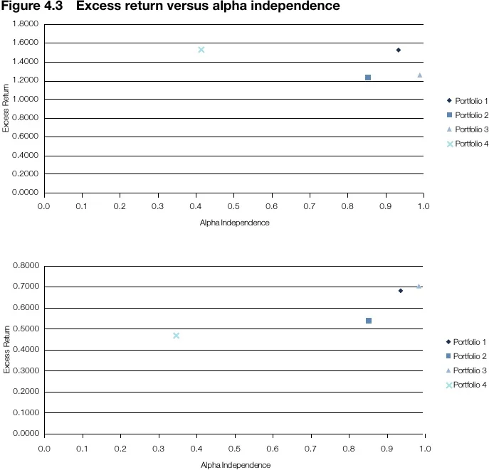
To summarise the results and present them in a more intuitive and appealing way, an alpha independence indicator was constructed for each portfolio for each period. The more independent the alpha, the more skill-driven the portfolio excess return-generation approach; the less independent the alpha, the more style-driven the portfolio excess return-generation approach.
In Figure 4.2, a plot was constructed with excess returns in the y-axis and alpha independence (1–R-squared) in the x-axis, giving a better picture of what has been analysed in this case study so far.
Conclusion
To assess the sources of return of asset managers, this chapter proposed a factor model approach based on linear regressions. The main conclusions are the following.
-
-
To begin with, there is another dimension to diversification, diversification among the defined risk factors, but the way in which excess returns are generated can also be diversified, and a new challenge would be to measure and find ways to balance style and skill-driven strategies.
-
-
-
It is not necessarily a good decision to get rid of a manager that produces lower excess returns if it generates excess returns in ways that are not likely to be replicated and are idiosyncratic to only that manager. Such a manager could be adding value, and might also be adding diversification to the aggregate portfolio.
-
-
-
The risk components and characteristics of a benchmark can be a defining factor for the way a manager approaches the generation of its excess returns. Theory suggests that, in a factor model approach, alpha generation is independent of the benchmark defined, but in practice the evidence suggests that when faced with different benchmarks, managers tend to change the approach according to the characteristics of each specific benchmark.
-
-
-
In our case study, we concluded that through the whole period there is consistency in the way portfolios 3 and 4 generate excess returns; while portfolio 4 uses a style-driven approach, portfolio 3 uses a skill-driven approach. Portfolios 1 and 2 redefine their approach according to the benchmark they have, but in general are either balanced or skewed to skill-driven strategies.
-
-
-
Additionally, there was diversification benefit from changing benchmarks; when faced with benchmark 1, portfolios 1 and 2 could be even considered redundant, but when benchmark 2 was incorporated the way of approaching excess returns generation was very different for such portfolios.
-
-
-
Finally, this is a valuable exercise for investment managers, particularly for reserve managers and official institution fund managers. In the public funds management world, it is not easy to justify the acquisition of expensive software or the consulting fees of technical experts. Therefore, an easy approach that does not rely on expensive software but is instead based on widely known statistical methods can be helpful. This understanding of performance may provide valuable information at a time of deciding on new benchmarks.
-
Appendix
In this analysis, evidence suggested that portfolios 1 and 2 are style-driven while portfolios 3 and 4 have some skill components that deviate its returns from their benchmarks returns.
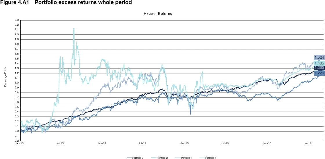
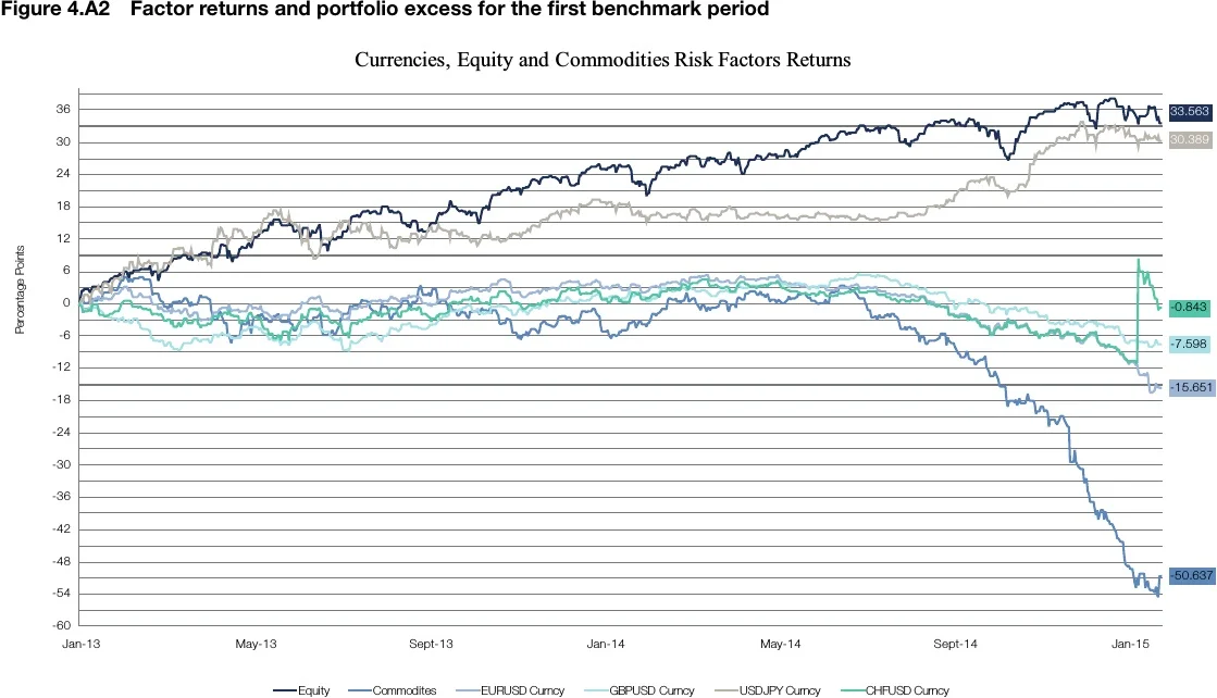
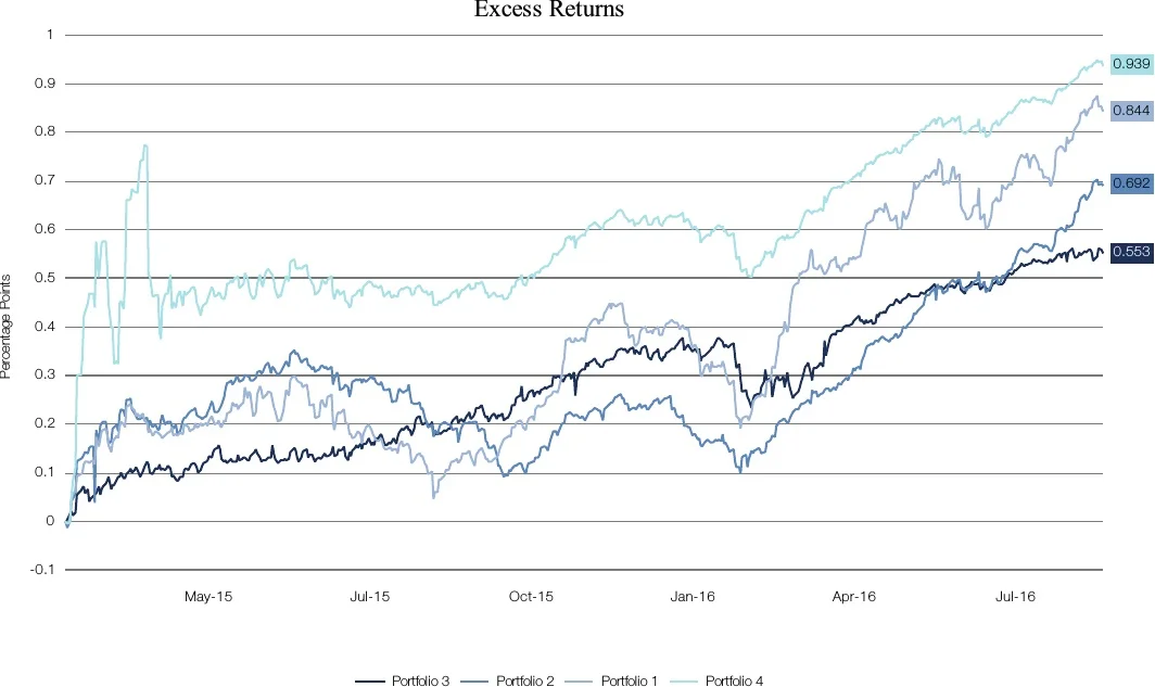
Figures 4A.1–4A.3 provide some additional charts of returns for the portfolios and the risk factors that help to further analyse how to link returns in the two benchmark periods to the returns of the factors. Figure 4A.1 is a chart of the returns of the four portfolios for the whole period, including both benchmarks; in Figure 4A.2, there are charts of returns for the first benchmark period and in Figure 4A.3 for the second benchmark period.

Only users who have a paid subscription or are part of a corporate subscription are able to print or copy content.
To access these options, along with all other subscription benefits, please contact info@centralbanking.com or view our subscription options here: subscriptions.centralbanking.com/subscribe
You are currently unable to print this content. Please contact info@centralbanking.com to find out more.
You are currently unable to copy this content. Please contact info@centralbanking.com to find out more.
Copyright Infopro Digital Limited. All rights reserved.
As outlined in our terms and conditions, https://www.infopro-digital.com/terms-and-conditions/subscriptions/ (point 2.4), printing is limited to a single copy.
If you would like to purchase additional rights please email info@centralbanking.com test test test
Copyright Infopro Digital Limited. All rights reserved.
You may share this content using our article tools. As outlined in our terms and conditions, https://www.infopro-digital.com/terms-and-conditions/subscriptions/ (clause 2.4), an Authorised User may only make one copy of the materials for their own personal use. You must also comply with the restrictions in clause 2.5.
If you would like to purchase additional rights please email info@centralbanking.com test test test


